
The Ackermann function is a well-known example of a function that grows extremely quickly and is used to demonstrate concepts in theoretical computer science and mathematical logic. It is defined using recursion, and unlike primitive recursive functions, it is not restricted to polynomial time, making it one of the earliest discovered examples of a computable function that is not primitive recursive.
Definition of the Ackermann Function
Recursive Nature
The Ackermann function is defined using recursion, with each case of the function reducing either one of its two parameters until it eventually reaches a base case. This recursive structure results in a function that grows far more quickly than typical recursive functions.
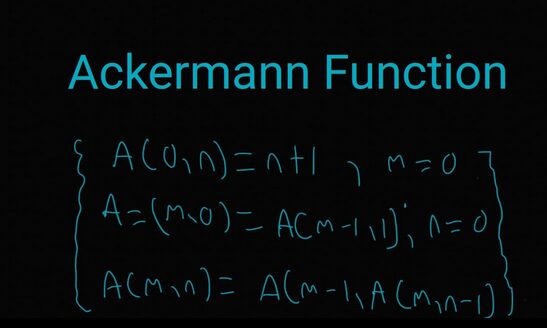
The Ackermann function is formally defined as:
[
A(m, n) =
\begin{cases}
n + 1 & \text{if } m = 0, \
A(m – 1, 1) & \text{if } m > 0 \text{ and } n = 0, \
A(m – 1, A(m, n – 1)) & \text{if } m > 0 \text{ and } n > 0.
\end{cases}
]
In this recursive structure:
- When ( m = 0 ), the function simply returns ( n + 1 ).
- When ( m > 0 ) and ( n = 0 ), the function reduces ( m ) by 1 and sets ( n ) to 1.
- When both ( m > 0 ) and ( n > 0 ), the function makes two recursive calls: first to reduce ( n ), and then to reduce ( m ) once ( n ) has been fully reduced.
Breakdown of the Function
Let’s break down what happens with different values of ( m ) and ( n ):
- When ( m = 0 ), the function simplifies to ( A(0, n) = n + 1 ), behaving similarly to basic addition.
- When ( m = 1 ), the function becomes ( A(1, n) = A(0, A(1, n – 1)) = n + 2 ), behaving like simple incrementing.
- When ( m = 2 ), the function becomes more complex: ( A(2, n) = 2n + 3 ), which behaves similarly to multiplication.
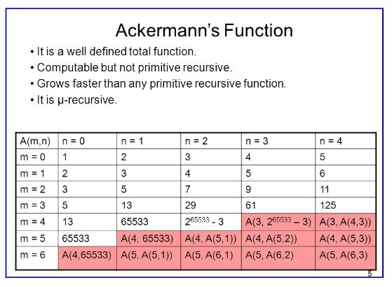
- When ( m = 3 ), the function starts behaving like exponentiation: ( A(3, n) = 2^{n+3} – 3 ).
- For ( m = 4 ) and beyond, the Ackermann function grows hyper-exponentially, making it difficult to represent the results even for small values of ( n ).
This nested recursion makes the Ackermann function an excellent demonstration of how small changes in input lead to dramatic increases in output, far beyond what primitive recursion can handle.
Theoretical Importance
Beyond Primitive Recursion
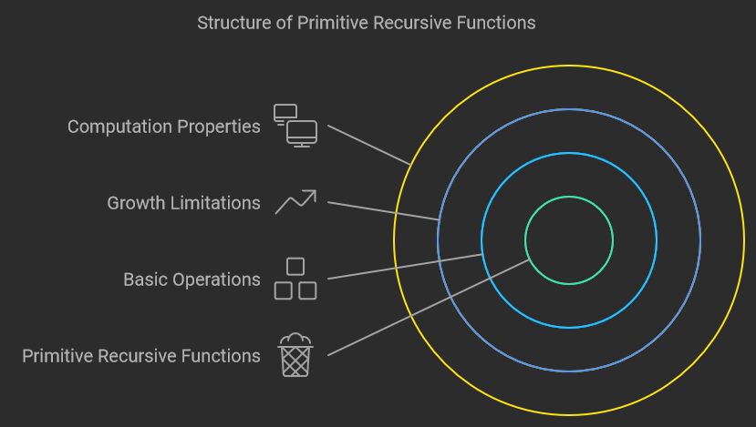
Primitive recursive functions are a class of functions defined using basic recursion and composition operations. These functions are limited in their growth potential, as they are built using simple operations like addition, multiplication, and bounded loops. They can be computed by a process that always terminates and runs in predictable time.
The Ackermann function, however, is an example of a total computable function that is not primitive recursive. While it can be computed for all inputs, its recursion is unbounded, meaning it does not fit within the restricted framework of primitive recursion. This is significant because the Ackermann function demonstrates a form of recursion that grows too rapidly for primitive recursive methods to handle. Essentially, it shows that not all computable functions are “simple” or predictable, as primitive recursion would suggest.
The distinction lies in the fact that primitive recursive functions can always be computed within a predictable number of steps, while the Ackermann function’s recursion grows so quickly that the number of steps becomes astronomical, even for small inputs. This challenges our understanding of what makes a function “computable” and highlights the limitations of using basic recursion for complex computations.
Relevance in Computability and Complexity Theory
The Ackermann function is significant in the fields of computability theory and complexity theory because it illustrates the boundaries between primitive recursive functions and more complex recursive functions. It serves as an early example of a total computable function that demonstrates the limitations of primitive recursion in terms of growth and efficiency.
In complexity theory, the Ackermann function is often used to demonstrate the difference between efficiently computable functions and those that, while computable, require a far greater number of computational steps. This distinction helps in understanding the computational costs of certain algorithms and functions. The function’s rapid growth makes it a practical example for demonstrating the theoretical limits of recursion and computation, particularly in problems that require immense processing power or memory.
Applications in Computer Science
In practical terms, the Ackermann function has been used in testing the limits of recursive algorithms, especially those that involve deep or unbounded recursion. Because of its explosive growth, the function can put significant strain on a system’s memory and processing capabilities, making it a useful benchmark for stress testing recursion in programming environments.
Some specific applications include:
- Evaluating Stack Efficiency: Since the Ackermann function causes extremely deep recursive calls, it can help evaluate the efficiency and depth-handling capacity of stack-based systems, especially in languages that rely heavily on recursion.
- Optimizing Tail Recursion: The function is also used to test optimization techniques for recursion, such as tail recursion, where compilers attempt to optimize recursive calls to prevent stack overflow. The Ackermann function can reveal how well a system can handle non-tail-recursive processes.
- Understanding Performance of Algorithms: In algorithm analysis, the function helps in illustrating how performance can degrade with non-linear recursive growth, offering a comparison between feasible algorithms and those that, while theoretically computable, become impractical to execute for large inputs.
The Ackermann function’s theoretical nature and extreme behavior make it a valuable tool for pushing the boundaries of what is computationally feasible and for understanding the scalability of recursive functions in real-world applications.
Conclusion
The Ackermann function stands out as a fascinating example in both mathematics and computer science due to its rapid, non-primitive recursive growth. It illustrates the limits of primitive recursive functions and plays a key role in understanding computability and complexity theory. The function’s extreme growth highlights how recursion can push the boundaries of computation, making it an essential tool for testing recursive algorithms and system performance.
In modern computer science, the Ackermann function continues to be relevant for its ability to challenge our understanding of recursion, algorithm efficiency, and system limitations. Despite its theoretical origins, its practical applications—especially in the realm of benchmarking and stress testing recursive systems—underscore its enduring significance in both academic and real-world contexts.
References for Further Reading
- Sipser, M. (2012). Introduction to the Theory of Computation.
A detailed look into recursive functions, computability, and complexity theory, including a discussion of the Ackermann function. - Sudkamp, T. (2006). Languages and Machines: An Introduction to the Theory of Computer Science.
This book explores recursive functions in depth, with examples like the Ackermann function to illustrate their computational properties. - Rosen, K. H. (2007). Discrete Mathematics and Its Applications.
A comprehensive source for understanding the mathematical structures behind recursive and non-recursive functions. - Wolfram MathWorld – Ackermann Function
https://mathworld.wolfram.com/AckermannFunction.html
A thorough online resource that provides detailed explanations and visualizations of the Ackermann function.
FAQ
1. What is the Ackermann function?
The Ackermann function is a mathematical function that grows very quickly and serves as an example of a total computable function that is not primitive recursive. It is used to demonstrate the limitations of primitive recursion and the extreme growth rate of certain recursive functions.
2. How is the Ackermann function defined?
The Ackermann function is defined recursively as follows:
[
A(m, n) =
\begin{cases}
n + 1 & \text{if } m = 0, \
A(m – 1, 1) & \text{if } m > 0 \text{ and } n = 0, \
A(m – 1, A(m, n – 1)) & \text{if } m > 0 \text{ and } n > 0.
\end{cases}
]
It computes values based on a set of recursive rules, where both ( m ) and ( n ) are reduced until a base case is reached.
3. Why is the Ackermann function important in computer science?
The Ackermann function is important because it illustrates the limits of primitive recursive functions and demonstrates how certain problems can lead to extremely rapid growth in computational complexity. It also serves as a benchmark for testing recursion and system performance in computer science.
4. How fast does the Ackermann function grow?
The Ackermann function grows incredibly fast. For small values of ( m ) and ( n ), the function behaves similarly to addition or multiplication, but as ( m ) increases, the function grows exponentially and even hyper-exponentially. For example, ( A(4, 2) = 2^{65536} – 3 ), a number far beyond standard notation.
5. What is the difference between the Ackermann function and primitive recursive functions?
Primitive recursive functions are restricted to basic recursion and bounded operations like loops, meaning their growth is predictable and limited. The Ackermann function, however, is an example of a non-primitive recursive function, meaning it exceeds the limitations of primitive recursion by growing much faster and without predictable bounds.
6. What are the applications of the Ackermann function in modern computing?
The Ackermann function is used to test recursive algorithms, evaluate system performance, and stress test stack memory in programming environments. Its extreme recursion helps developers understand how systems handle deep recursive calls and optimize recursion handling in programming languages.
7. How does the Ackermann function relate to computability and complexity theory?
In computability theory, the Ackermann function shows that not all computable functions can be computed using primitive recursion. In complexity theory, it is used to demonstrate the limitations of computational efficiency and highlight the challenges of solving certain problems due to rapid recursive growth.
8. Is the Ackermann function used in real-world programming?
While the Ackermann function is primarily theoretical, it has practical applications in testing system limitations, especially in recursion-heavy algorithms. It’s also used as a benchmark for evaluating the effectiveness of optimization techniques like tail-recursion in programming languages.
9. Can the Ackermann function be computed by modern computers?
For small inputs, modern computers can compute the Ackermann function. However, for larger values, the function grows so quickly that it becomes impossible to compute due to memory and time constraints, even on advanced systems.